Double Integrals Over Rectangles

Consider a function $f(x)$ defined for $x \in [a,b].$ We divide the interval $[a,b]$ into $n$-subintervals $\left[x_i,x_{i+1}\right]$ of equal width $\Delta x = (b-a)/n$ and we choose sample points $x_i^*$ in these subintervals to form the Riemann sum \[ \sum_{i=0}^{n-1}f\left(x_i^*\right)\Delta x. \] Then we take the limit of such sums as $n\to \infty$ to obtain the definite integral of $f$ from $a$ to $b:$ \[ \displaystyle \int_a^b f(x)dx = \lim_{n \to \infty} \sum_{i=0}^{n-1} f\left(x_i^*\right)\Delta x \] For the special case where $f(x)\geq 0,$ the Riemann sum can be interpreted as the sum of the areas of the approximation rectangles, and $\int_a^b f(x)dx$ represents the area under the curve $y=f(x).$

In a similar way we consider a function of two variables defined on a closed rectangle

We first suppose that $f(x,y)\geq 0.$ The graph of $f$ is a surface with equation $y = f(x,y).$ Let $V$ be region that lies above $R$ and under the graph of $f,$ that is,

Our goal here is to find the volume of $V.$

Divide $R$ into subrectangles by dividing $[a,b]$ into $m$ subintervals $[x_{i-1},x_i]$, each of width $$\Delta x =\frac{b-a}{m}$$ and $[c,d]$ into $n$ subintervals $[y_{i-1},y_i]$ of equal width $$\Delta y = \frac{d-c}{n}.$$

Combining these gives a rectangular grid $R_{ij}$ with subrectangles each of area $\Delta A= \Delta x\Delta y.$ In each subrectangle take any point $P_{ij}$ with co-ordinates $\left(x_{ij}^*, y_{ij}^*\right).$

The volume of the box with base the rectangle $\Delta A$ and height the value of the function $f(x,y)$ at the point $P_{ij}$ (so the box touches the surface at a point directly above $P_{ij}$) is \[ V_{ij} = f\left(x_{ij}^*, y_{ij}^*\right)\Delta A \]

Then for all the subrectangles we have an approximation to the required volume $V$: \[ V\approx \sum_{i=1}^m\sum_{j=1}^n f\left(x_{ij}^*, y_{ij}^*\right) \Delta A, \] the double Riemann sum.

Let $\Delta x \to 0 $ and $\Delta y \to 0,$ i.e., $m\to \infty$ and $n\to \infty,$ then we define the volume to be \[ V= \lim_{m,n\to \infty} \sum_{i=1}^m\sum_{j=1}^n f\left(x_{ij}^*, y_{ij}^*\right) \Delta A, \] if the limits exist, and we write this as $$\ds \iint_Rf(x,y)~dA. $$

We call $f$ integrable if the limit exists. Note that every continuous function is integrable.

Historical note

The exhaustion method for computing volumes in calculus is an ancient technique, dating back to Archimedes, that approximates a given volume by inscribing and circumscribing a sequence of simpler shapes (e.g., prisms or cylinders) whose volumes can be precisely computed. The key idea is to take an increasing number of these shapes, making their total volume approach the true volume of the solid.

In modern calculus, this idea evolved into Riemann integration and is formalized through definite integrals. So in essence, to compute the volume of a solid using the exhaustion method:

1. Slice the solid into thin sections (e.g., disks, boxes, or shells).
2. Approximate each section's volume using a simple geometric shape.
3. Sum the volumes of these sections to form an approximation.
4. Take the limit as the number of slices increases and their thickness approaches zero.

Iterated Integrals

It is often challenging to evaluate single integrals directly using the definition of an integral. However, the Fundamental Theorem of Calculus offers a more straightforward approach. Evaluating double integrals from first principles is even more complex, but we can simplify the process by expressing a double integral as an iterated integral, allowing us to compute it by evaluating two single integrals sequentially.

We define $\displaystyle \int_c^df(x,y)~dy$ to mean that $x$ is fixed and $f(x,y)$ is integrated with respect to $y$ from $y=c$ to $y=d$. So \[ A(x) = \int_c^df(x,y)~dy \] is a function of $x$ only. If we now integrate $A(x)$ with respect to $x$ from $x=a$ to $x=b$ we have

This is called the iterated integral.

Similarly, we have the iterated integral

In this case we first integrate with respect to $x$ (holding $y$ fixed) from $x=a$ to $x=b$ and then we integrate the resulting function of $y$ with respect to $y$ from $y=c$ to $y=d.$ Notice that in both equations (\ref{iter-int-01}) and (\ref{iter-int-02}) we work from the inside out.

Fubini's Theorem

Observe that in Example 1, we arrived at the same result regardless of whether we integrated first with respect to $y$ or $x.$ More generally, the two iterated integrals in equations (\ref{iter-int-01}) and (\ref{iter-int-02}) are always equal, meaning the order of integration does not affect the outcome. The following theorem provides a practical approach for evaluating a double integral by expressing it as an iterated integral in either order.

The following theorem gives a practical method for evaluating a double integral by expressing it as an iterated integral (in either order).

Of course, Fubini's theorem can be generalized to the case where $f$ is not necessarily continuous.

In the special case where $f(x,y),$ can be factored as the product of a function of $x$ only and a function of $y$ only, the double integral of $f$ can be written in a particularly simple form. That is, suppose that $f(x,y) = g(x)h(y)$ and $R= [a,b]\times[c,d].$ Then Fubini's Theorem gives

In the inner integral, $y$ is a constant, so $h(y)$ is a constant and we can write

since $\int_a^b g(x)~dx$ is a constant. Hence, if $f$ can be written as the product of two integrals:

Double Integrals Over General Regions

In this section, we have two main goals: first, to define the double integral of a function $f(x, y)$ over regions $D$ that are more general than rectangles; second, to develop a method for evaluating this type of integral. To achieve this, we will introduce two specific types of subsets in the $xy$-plane and then extend the concept of the double integral to these regions.

To define a double integral over a non-rectangular region $D$, we consider a rectangular $R$ which encloses $D$ and define

Then we can define the double integral of $f(x,y)$ over $D$ by \[ \iint_D f(x,y) dA= \iint_R F(x,y)dA \]

1. Chop $R$ into subrectangles,
2. Compute $F(x^*,y^*)\Delta A$ for each rectangle contained in $R,$
3. Add up the contributions from all subrectangles, and
4. Take a limit as we chop $R$ into smaller and smaller pieces.

Then

However, this does not really tell us how to compute the double integral over $D.$ 😥

So we need to consider an alternative way of calculating the volume below a surface above a rectangle $R,$ which can be easily generalized to compute double integral over a general region. Here we need to introduce two types of plane regions.

A plane region $D$ is of type I if it lies between the graph of two continuous functions of $x.$ That is $$D=\left\{ (x,y) ~|~ a \leq x\leq b, g_1(x) \leq y \leq g_2(x) \right\}.$$

In practice, to evaluate $\iint_D f(x,y)dA$ where $D$ is a region of type I we have \[ \iint_D f(x,y)~dA = \int_a^b \int_{g_1(x)}^{g_2(x)} f(x,y) ~dy~dx \]

A plane region is of type II if it can be expressed by $$D=\left\{ (x,y) ~|~ c \leq y\leq d, h_1(y) \leq x \leq h_2(y) \right\}.$$

In practice, to evaluate $\iint_D f(x,y)dA$ where $D$ is a region of type II we have \[ \iint_D f(x,y)dA = \int_c^d \int_{h_1(y)}^{h_2(y)} f(x,y) ~dx~dy \]

It is often possible to represent a type I region as a union of type II regions, or a type II region as a union of type I regions. Why would we want to do that? In some cases, it may only be possible to integrate a function one way but not the other.

One thing to observe from the previous example is that when treating the double integral as a type II region, the calculations become slightly more complex. If you encounter this while computing a double integral, a useful strategy is to switch the region from type I to type II or vice versa, depending on your initial setup.

In the following example, we see how it is sometimes necessary to change the order of integration in order to evaluate the integral.

Properties of double integrals

For rectangular regions $R$ the first three properties can be easily proved. For general regions the properties follow from Definition 1.

1. $\displaystyle \iint_R \left(\,f\pm g\right)dA = \iint_Rf~dA \pm \iint_R g~dA$
2. $\displaystyle \iint_R c~f~dA = c\iint_Rf~dA$
3. If $f(x,y)\geq g(x,y)$ for all $(x,y)\in R$ then
   $$\displaystyle \iint_R f~dA \geq \iint_Rg~dA$$
4. If $R= R_1 \cup R_2,$ where $R_1$ and $R_2$ are regions that don't overlap except perhaps on their boundaries, then
   $$\displaystyle \iint_R f~dA = \iint_{R_1}f~dA + \iint_{R_2}f~dA$$

Double Integrals in Polar Coordinates

For annular regions with circular symmetry, rectangular coordinates are difficult. It can be more convenient to use polar coordinates. The following diagram explains the relationship between the polar variables $r,$ $\theta$ and the usual rectangular ones $x, y.$

For polar coordinates, we have \[ x = r\cos \theta, \quad y = r \sin \theta. \]

Consider the volume of a solid beneath a surface $z = f(x,y)$ and above a circular region in the $xy$ plane.

We divide the region into a polar grid as in the following diagram:

We first approximate the area of each polar rectangle as a regular rectangle. We do this as follows. Choose a point $P$ inside each polar rectangle in the polar grid.

Let $P = (x^*, y^*)$ or in polar coordinates $P = (r^*, \theta^*)$ , where \[ x^* = r^*\cos \theta^*, \;\; y^* = r^* \sin \theta^*. \]

The area of the polar rectangle containing $P$ can be approximated as $r^*~\Delta \theta ~\Delta r$.

Therefore the volume under the surface and above each polar rectangle can be approximated as

Here $f\left( r^*\cos \theta^*, r^* \sin \theta^* \right)$ is the value of the function at the point $P$, which is also the height of the box used in the approximation.

To obtain an approximation for the entire volume below the surface, we sum over the entire polar grid:

The double integral in rectangular coordinates is then transformed as follows:

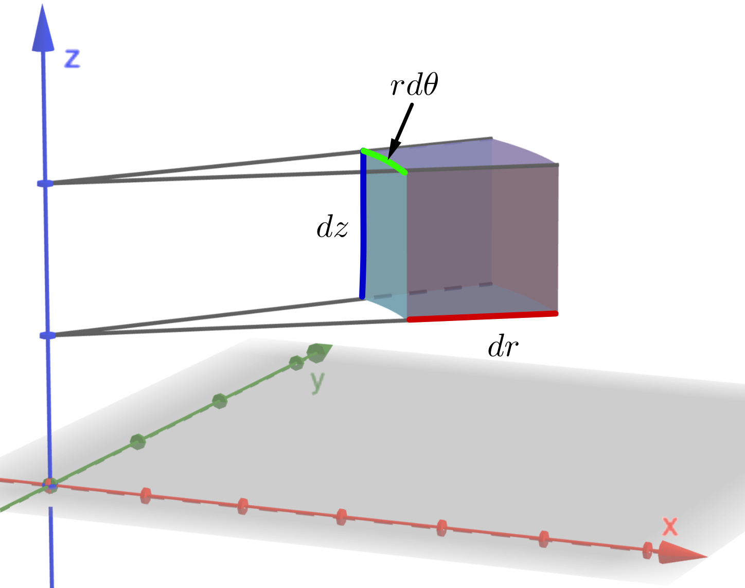
The formula in (\ref{iint-polar}) says that we can convert from rectangular to polar coordinates in a double integral by writing $x=r\cos\theta $ and $y= r\sin \theta$ using the appropriate limits of integration for $r$ and $\theta$ and replacing $dA$ by $r ~dr ~d\theta.$ Just be careful! Don't forget to add the factor $r$ on the right side. A classical method for remembering this is shown in Figure 14, where the "infinitesimal" polar rectangle can be thought of as an ordinary rectangle with dimensions $r \,d\theta$ and $dr$ and therefore has "area" $dA= r\, dr \,d\theta.$

Triple Integrals

Similarly to how we defined single integrals for functions of one variable and double integrals for functions of two variables, we can define triple integrals for functions of three variables. Let's first consider the simplest case where the function $f(x,y,z)$ is defined on a rectangular box.

First we divide $B$ into sub-boxes. We do this by dividing the interval $[a,b],$ into $l$ subintervals $\left[x_i, x_{i+1}\right]$ of equal width $\Delta x,$ dividing $[c,d]$ into $m$ subintervals of width $\Delta y,$ and dividing $[r,x]$ into $n$ subintervals of width $\Delta z.$ The planes through the endpoints of these subintervals parallel to the coordinate planes divide the box $B$ into lmn sub-boxes

Each sub-box has volume $\Delta V = \Delta x \Delta y \Delta z.$

Then we form the triple Riemann sum

where $\left(x_{ijk}^*, y_{ijk}^*, z_{ijk}^*\right)\in B_{ijk}.$ Similarly to the definition of a double integral, we defined the triple integral as the limit of the triple Riemann sums:

Just as for double integrals, the practical method for evaluating triple integrals is to express them as iterated integrals as follows.

The first iterated integral on the right side of Fubini's Theorem means that we integrate first with respect to $x$ (keeping $y$ and $z$ fixed), then we integrate with respect to $y$ (keeping $z$ fixed), and finally we integrate with respect to $z.$ There are six possible orders altogether, all of which give the same value.

Now we define the triple integral over a general bounded region $R$ in the three-dimensional space (a solid) similar to the procedure that we used for double integrals.

A solid region $R$ is said to be of type 1 if it lies between the graphs of two continuous functions of $x$ and $y,$ that is,

where $D$ is the projection of $R$ onto the $xy$-plane. In this case we the upper boundary of the solid $R$ is the surface with equation $z=s(x,y)$ while the lower boundary is the surface $z=r(x,y).$

Thus we have that if $R$ is a type 1 region, then

The inner integral on the right side of the previous equation means that if $x$ and $y$ are held fixed, and therefore $r(x,y)$ and $s(x,y)$ are regarded as constants, while $f(x,y,z)$ is integrated with respect to $z.$

In particular, if the projection $D$ of $R$ onto the $xy$-plane is a type I plane region, then

and so

If, on the other hand, $D$ is a type II plane region, then

and in this case we have

Now, a solid region $R$ is of type 2 if it is of the form

where, in this case, $D$ is the projection of $R$ onto the $yz$-plane. Then we have

Finally, a solid region $R$ is of type 3 if it is of the form

where, in this case, $D$ is the projection of $R$ onto the $xz$-plane. For this type of region we have

For each of the equations (\ref{type-1}) and (\ref{type-3}) there may be two possible expressions for the integral depending on whether $D$ is a type I or type II plane region, similar to to Equations (\ref{type-1-type-I}) and (\ref{type-1-type-II}).

Express $I= \ds\int_{0}^{1}\int_{\sqrt{x}}^{1}\int_{0}^{1-y} f(x,y,z)~dz~dy~dx$ in the orders $dz~dx~dy$ and $dy~dz~dx.$

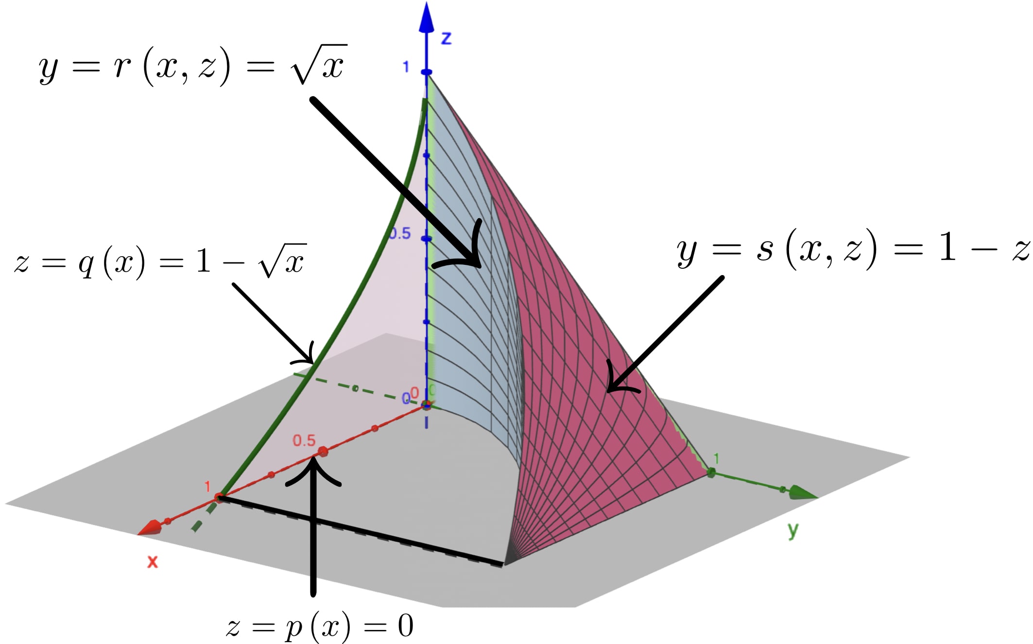
We can write

\begin{eqnarray*} I = \int_{x=0}^{x=1}\int_{y=\sqrt{x}}^{y=1}\left[ \int_{z=0}^{z=1-y} f ~dz \right]dy~dx &=& \iiint_{R} f(x,y,z)~dz~ dy~dx \end{eqnarray*}

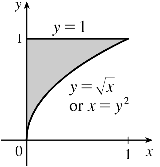
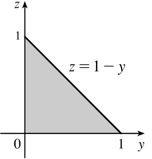
where $R= \left\{(x,y,z)~|~ 0\leq x\leq 1,~ \sqrt{x}\leq y \leq 1,~ 0\leq z\leq 1-y \right\}.$ This description will enable us to write projection onto different planes.

First, let's express $I$ in the order $dz~dx~dy.$

\begin{eqnarray*} I = \int_{x=0}^{x=1}\int_{y=\sqrt{x}}^{y=1}\left[ \int_{z=0}^{z=1-y} f ~dz \right]dy~dx &=& \iint_{D}\left[ \int_{z=0}^{z=1-y} f ~dz \right]dy~dx \end{eqnarray*}

Here $D$ is the projection of the region on the plane $xy.$ Then

\begin{eqnarray*} I &=& \iint_{D}\left[ \int_{z=0}^{z=1-y} f ~dz \right] dx~dy \\ &=& \int_{y=0}^{y=1}\int_{x=0}^{x=y^2}\left[ \int_{z=0}^{z=1-y} f ~dz \right]dx~dy \end{eqnarray*}

The original integral was of type I. But when we change the order $dy~dx$ to $dx~dy,$ we have now a type II integral.

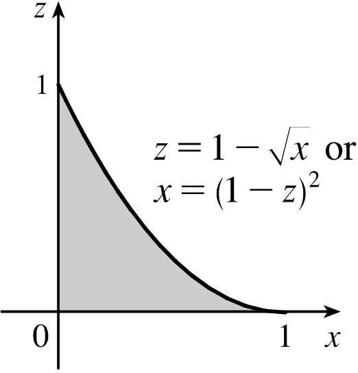
Now, let's express $I$ in the order $dy~dz~dx.$

\begin{eqnarray*} I = \int_{x=0}^{x=1}\int_{y=\sqrt{x}}^{y=1}\left[ \int_{z=0}^{z=1-y} f ~dz \right]dy~dx &=&\int_{x=0}^{x=1}\left[ \int_{y=\sqrt{x}}^{y=1} \int_{z=0}^{z=1-y} f ~dz~ dy\right]dx \\ &=& \int_{x=0}^{x=1}\bigg[ \int_{z=0}^{z=1-\sqrt{x}} \int_{y=\sqrt{x}}^{y=1-z} f~\bigg]dx \\ &=& \int_{x=0}^{x=1} \int_{z=0}^{z=1-\sqrt{x}}\left[ \int_{y=\sqrt{x}}^{y=1-z} f~dy \right] dz~dx \\ &=& \iint_D \left[ \int_{y=\sqrt{x}}^{y=1-z} f~dy \right] dA \end{eqnarray*}

Here $D$ is the projection of the region on the plane $xz.$

In any case, we have that

\begin{eqnarray*} I = \int_{x=0}^{x=1}\int_{y=\sqrt{x}}^{y=1}\left[ \int_{z=0}^{z=1-y} f ~dz \right]dy~dx = \int_{x=0}^{x=1} \int_{z=0}^{z=1-\sqrt{x}} \left[ \int_{y=\sqrt{x}}^{y=1-z} f~dy \right] dz~dx \end{eqnarray*}

There are three more possible orders in which we can integrate. Below you can see all the possible combinations with their corresponding projections on the $xy,$ $yz,$ and $xz$ planes.

	$ \quad \ra \quad \displaystyle \int_0^1$ $\displaystyle \int_{\sqrt{x}}^{1}$ $\displaystyle \int_{0}^{1-y} $ $f$ $ dz$ $dy$ $dx$ $ \,= $ $\displaystyle \int_0^1 $ $\displaystyle \int_{0}^{y^2} $ $\displaystyle \int_{0}^{1-y}$ $f$ $ dz$ $dx$ $dy$
	$\quad \ra \quad \displaystyle \int_0^1$ $\displaystyle \int_{0}^{1-z}$ $\displaystyle \int_{0}^{y^2}$ $f$ $dx$ $dy$ $dz$ $ \,= $ $\displaystyle \int_0^1$ $\displaystyle\int_{0}^{1-y}$ $\displaystyle\int_{0}^{y^2}$ $f$ $ dx$ $dz$ $dy$
	$\quad \ra \quad \displaystyle \int_0^1$ $\displaystyle \int_{0}^{1-\sqrt{x}}$ $\displaystyle \int_{\sqrt{x}}^{1-z}$ $f$ $ dy$ $dz$ $dx$ $ \,= $ $\displaystyle \int_0^1 $ $\displaystyle \int_{0}^{(1-z)^2}$ $\displaystyle \int_{\sqrt{x}}^{1-z}$ $f$ $ dy$ $dx$ $dz$

If you want, you can explore all the projections in the following applet:

Triple Integrals in Cylindrical Coordinates

Sometimes it is useful to use cylindrical coordinates in order to simplify the integral. This involves the transformation

We now aim to calculate a small element of volume of a cylindrical shell. This will then show how in a triple integral we can transform from rectangular coordinates to cylindrical coordinates by substituting the transformation (\ref{cylindrical-coord}) and by making the change \[ dx~dy~dz\rightarrow r~dr~d\theta ~dz \]

The important result is that the triple integral in rectangular coordinates transforms as follows:

Triple Integrals in Spherical Coordinates

Sometimes it is useful to use spherical coordinates in order to simplify the integral. This involves the transformation

We now aim to calculate a small element of volume of a spherical shell. This will then show how in a triple integral we can transform from rectangular coordinates to spherical coordinates by substituting the transformation (\ref{spherical-coord}) and by making the change \[ dx~dy~dz\rightarrow r^2\sin \phi ~dr~d\theta ~d\phi \]

Consider the following diagram.

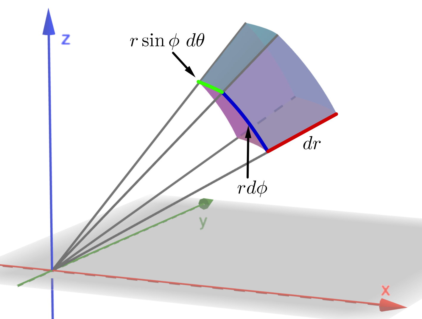
The important result is that the triple integral in rectangular coordinates transforms as follows: